LLRFLibsPy Algorithms#
General Information#
The reference articles for most algorithms used in LLRFLibsPy are documented in code pages (see Modules).
Here we collect additional info about the algorithms used in the library.
rf_sysid Functions#
prbs#
The routine generates a Pseudorandom Binary Sequence (PRBS), which can be used as a stimuli signal for system identification. Note that the number of point \(n\) should satisfy
with \(k\) an integer, to achieve a constant magnitude in the Power Spectral Density (PSD) of the resulting time series.
etfe#
The ETFE algorithm estimates the frequency response of the system using the Discrete Fourier Transform (DFT) of the output (\(y\)) and input (\(u\)), given by
Here \(U\) and \(Y\) are the DFT of \(u\) and \(y\), respectively. The DFT is calculated with \(N\) samples sampled at frequency \(f_s\). There are two methods implemented to improve the performance of ETFE:
Using repeated inputs (with \(r\) batches of data by repeating the same input series by \(r\) times) and making average to reduce the effects of measurement noise.
Remove the data in the transient of the system response (i.e., the first several batches of data).
cav_drv_est#
This function estimates the waveforms of the cavity drive signal (\({{{\bf{v}}_{for}}}\)) and reflected signal (\({{{\bf{v}}_{ref}}}\)) using the cavity probe signal (\({{{\bf{v}}_{C}}}\)) as reference. The input coupling factor (\(\beta \)), half-bandwidth (\({\omega _{1/2}}\)), and detuning (\({\Delta \omega }\)) should be given. The algorithm uses the following cavity equation with voltage drives (Eq. (3.31) of LLRF Book [1]):
with the beam drive voltage \({{{\bf{v}}_{b0} = 0}}\). The forward and reflected voltage waveforms are calculated as
The implementation has used the discretized cavity equation to avoid directly calculating the derivative of the cavity voltage.
cav_par_pulse#
The implementation actually uses the polar differential equations of the cavity given by Eq. (4.24) in the LLRF Book.
The derivative is calculated with the gradient function of numpy, which is sensitive to the measurement noise.
In the example code, one can compare the result of this function with that of cav_par_pulse_obs, which avoids
calculating the derivative and therefore, gives more smooth results.
cav_par_pulse_obs#
This function uses a disturbance observer to estimate the cavity voltage (smoothen the cavity probe signal) and a general disturbance term. From the general disturbance term, the cavity half-bandwidth and detuning at each time step can be estimated. The algorithm is described in the referred paper. The major benefit of the observer is that we can avoid calculating the derivatives and obtain less noisy results. Note that the beam drive term (calibrated to the same reference plane as the cavity probe signal) should be input to calculate the time-varying half-bandwidth and detuning if the beam is present.
cav_beam_pulse_obs#
Similar to the cav_par_pulse_obs function, this function calculates the waveform of the beam drive voltage given
the cavity probe, forward signals and the intra-pulse half-bandwidth and detuning (e.g., calculated when the beam
is off). Here we assume that the cavity voltage with the beam present is well controlled to be the same as the case
without beam. Only in this case, the half-bandwidth and detuning of the cavity during the RF pulse can be assumed
unchanged after injecting the beam.
iden_impulse#
This function estimates the impulse response of a system using its input and output signals. Complex signals are allowed for the RF system with its input and output as phasors representing the signals’ complex envelopes. The relationship between the input \(u\), output \(y\), and the system’s impulse response \(h\) is described by Eq. (4.41) of the LLRF Book. Here we model the system as a Finite Impulse Response (FIR) filter, therefore, the order should be large enough to cover most of the significant elements in the impulse response \(h\).
rf_calib Functions#
calib_vprobe#
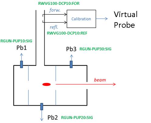
One example to apply the virtual probe calibration is for the SwissFEL Gun, whose probe if strongly affected by the mechanical vibrations caused by the cooling system. As shown in the Figure 1, the forward and reflected signals picked before the Gun cavity input coupler are calibrated with two complex coefficients (\(\bf{m}\) and \(\bf{n}\)) to match one of the cavity probe signal (see the equation in the function description above).
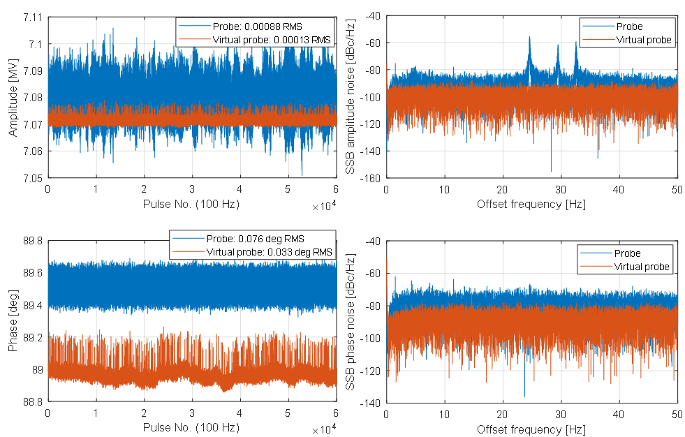
After calibration, the virtual probe signal was used as the input for RF feedback. Figure 2 compares the amplitudes and phases of the physical probe (Pb1) and virtual probe. It can be seen that the resonance peaks in the probe amplitude (caused by the mechanical vibrations applied to the probe antenna) is not visible in the virtual probe signal.
calib_ncav_for_ref#
The implementation used a simplified algorithm compared to the one described in the Sect. 9.3.5 of the LLRF Book.
This simplification benefits from the assumption that the loaded Q and detuning of the cavity are constant. First,
the theoretical cavity forward and reflected signals are estimated with the cav_drv_est function. Then, we estimate
the coefficients \(\bf{m} = \bf{a} + \bf{b}\) and \(\bf{n} = \bf{b} + \bf{d}\) using the calib_vprobe function. After that, we estimate \(\bf{a}\) and \(\bf{b}\) based on
the estimated theoretical forward signal and the measured forward and reflected signals (also using calib_vprobe –
use its feature of least-square fitting). Finally, all the four parameters \(\bf{a}\), \(\bf{b}\), \(\bf{c}\), and \(\bf{d}\) are calculated.
calib_scav_for_ref#
The implementation is slightly different compare to the algorithm described in the Sect. 9.3.5 of the LLRF Book. The major difference is the method to calculate the parameter \(\bf{a}\). In this implementation, \(\bf{a}\) is calculated using the estimated theoretical forward signal around the end of the RF pulse, where the cavity half-bandwidth and detuning is assumed to be the same as the parameter values input to the function.
for_ref_volt2power#
When using this function (and other functions requiring specification of machine), one must notice the difference
of the definitions of the normalized effective shunt impedance in storage rings and Linacs. In a Linac, the normalized
effective shunt impedance (\(r/Q\)) of a standing-wave cavity is defined as
where \(V_{acc}\) is the accelerating voltage taking into account the transit time factor, \(P_{cav}\) is the RF power dissipated in the cavity wall, \(\omega _0\) is the cavity resonance frequency (angular frequency), and \(W\) is the stored electromagnetic field energy in the cavity. Here \(r\) is the effective shunt impedance. In a storage ring, we have the following definition:
Therefore, we have the following relation between the \(R/Q\) given in storage-ring cavity specifications and the \(r/Q\) given in Linac cavity specifications:
In the LLRF Book, the loaded resistance \(R_L\) (Sect. 3.3.1) is defined following the Linac convention. It can be rewritten as follows in either Linac or storage-ring conventions:
Now let’s workout the method how to convert the forward/reflected voltages (already calibrated to physical units) into powers. The relation between the forward (reflected) current phasor and voltage phasor is
where \(\beta\) is the input coupling factor of the cavity. Therefore, the forward (reflected) power can be calculated from the forward (reflected) voltage as
Here * is the conjugate of the phasor. Note that for superconducting cavities, \(\beta\) is much larger than 1, then the terms with \(\beta\) can be neglected and we reach the Eq. (9.35) of the LLRF Book.
rf_control Functions#
ss_discrete#
This function converts the continuous state-space equation
into a discrete state-space equation as
where \(k\) is the index of the samples. If enabled, the frequency response of the continuous and discrete state-space equations can be plot for comparison. The parameters should be tuned to match the discrete system frequency response to the continuous system frequency response as much as possible.
basic_rf_controller#
The phasor transfer function of the basic RF controller is given by
This is a Proportional-Integral (PI) controller with frequency notches at \(\omega _{notch,i}, {\quad} i = 1,…,n\). This controller is used in an I/Q control loop. It accepts a complex input (\(I + jQ\)) and produces a complex output actuating on the I and Q channels via its real and imaginary components, respectively. The parameters are described as follows:
\(K_P\): proportional gain
\(K_I\): integral gain
\(g_i\): max gain of the ith notch filter
\(\omega _{1/2,i}\): half bandwidth of the \(i\)th notch filter
\(\omega _{notch,i}\): frequency to be suppressed by the \(i\)th notch filter
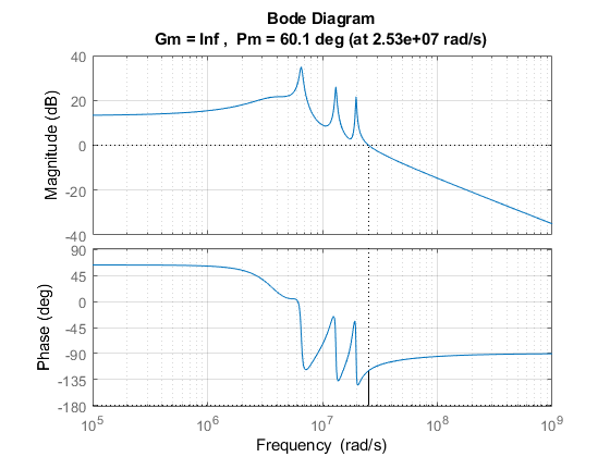
Note that we apply notches at both sidebands with frequency offsets of \( \pm \omega _{notch,i}\). If it is clear that the disturbance to be suppressed appears only at one sideband, the notch filter at the other sideband can be discarded. The returned controller is in the format of state-space equation. Figure 3 shows the open-loop bode plot of an RF control loop consisting of a cavity and a basic RF controller. The cavity parameters are: resonance frequency = 500 MHz, half-bandwidth = 281.7 kHz, detuning = 2 * 281.7 kHz. The controller is a P controller with \(K_P\) = 10 and with notches at 1*, 2*, and 3*1.04 MHz.
loop_analysis#
The open-loop transfer function is constructed by cascading the system state-space equation (AG, BG, CG, DG) and the
controller state-space equation (AK, BK, CK, DK). The frequency response of the open loop can be used to construct
the bode-plot and Nyquist plot, with which the closed-loop stability and the phase/gain margins can be examined.
rf_det_act Functions#
noniq_demod#
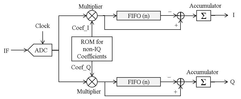
This function demodulates the input waveform into I and Q components. The algorithm follows Eq. (5.22) of the LLRF Book. However, the implementation applies some tricks originally aiming at implementing this algorithm in FPGA. See Figure 4. The “non-IQ Coefficients” are
Note that in Figure 4, all the components are synchronized by the same clock as ADC.
asyn_demod#
This function demodulates the input raw waveform using the reference tracking method. Note that the implementation here only works for buffered waveforms. You need to input the whole waveform of the signal to be demodulated and the waveform of the reference signal sampled at the same time. Modifications are needed if this algorithm is applied to streamed samples (e.g., in FPGA). Here summarize the key points in the implementation:
The carrier (IF) frequency of the signal is estimated via FFT.
The function
twop_demodis used to demodulate both waveforms.The reference phase is used to detect the phase slope (representing the error of the estimated carrier frequency), which is used to correct the phase of the signal to be demodulated.
self_demod_ap#
For a real time-domain signal \(y(t)\), its Hilbert transform is defined as
Then for signal \(y(t)\), a complex signal can be constructed as
From it the amplitude and phase of the signal \(y(t)\) can be calculated as
This function can be used to estimate the amplitude and phase of a waveform without knowing the sampling parameters such as the carrier frequency or the sampling frequency. With the estimated amplitude and phase, the amplitude and phase jitter of the waveform can be examined.
rf_noise Functions#
gen_noise_from_psd#
This function generates a time series with its PSD spectrum the same as that given by input parameters. The implementation follows the algorithm below:
Derive the PSD at the \(N\) frequency points (corresponding to \(N\) data points, covering from \(f_s/N\) to \(f_s\)) by linearly interpreting the given PSD spectrum with the frequency and PSD both in the logarithm scale.
From the interpreted PSD, calculate the DFT magnitude of the positive frequencies by inversing the formula of the periodogram method. See Eq. (6.15) of the LLRF Book. Then derive the complex DFT at positive frequencies by assigning a random phase to each point.
Construct the full DFT from 0 to \(f_s\) (the DFT from \(f_s/2\) to \(f_s\) is the conjugate of the image frequencies from \(f_s/2\) down to 0), and calculate the time series with the inversed DFT (IDFT).
calc_rms_from_psd#
This function interprets the given PSD spectrum (similar to gen_noise_from_psd) and calculates the RMS jitter by
integrating the noise power from freq_start to different ending frequencies up to freq_end.
rf_sim Functions#
sim_ncav_step_simple#
This function discretize the cavity equation with the Euler method. The accuracy will become bad if the sampling time \(T_s\) is close to the time constant of the cavity dynamics (e.g., transient caused by large detuning or the dynamics of pass-band modes).
References#
[1] S. Simrock and Z. Geng, Low-Level Radio Frequency Systems, Springer, 2022. https://link.springer.com/book/10.1007/978-3-030-94419-3